Math Into Code

Semi-interactive code for simulations in the NVT ensemble according to the Metropolis’ acceptance/rejection criteria derived from the detailed balance condition of the ergodic markov chain proposed.

The environment consists of a fixed-size simulation box centered in the origin, filled with spherical molecules based on the density of the system. Their interaction is according to either a Lennard-Jones or Square-Well potential (implementation of additional potentials is straightforward) in the reduced unit’s system.

New states are generated by random displacements of the molecules position,

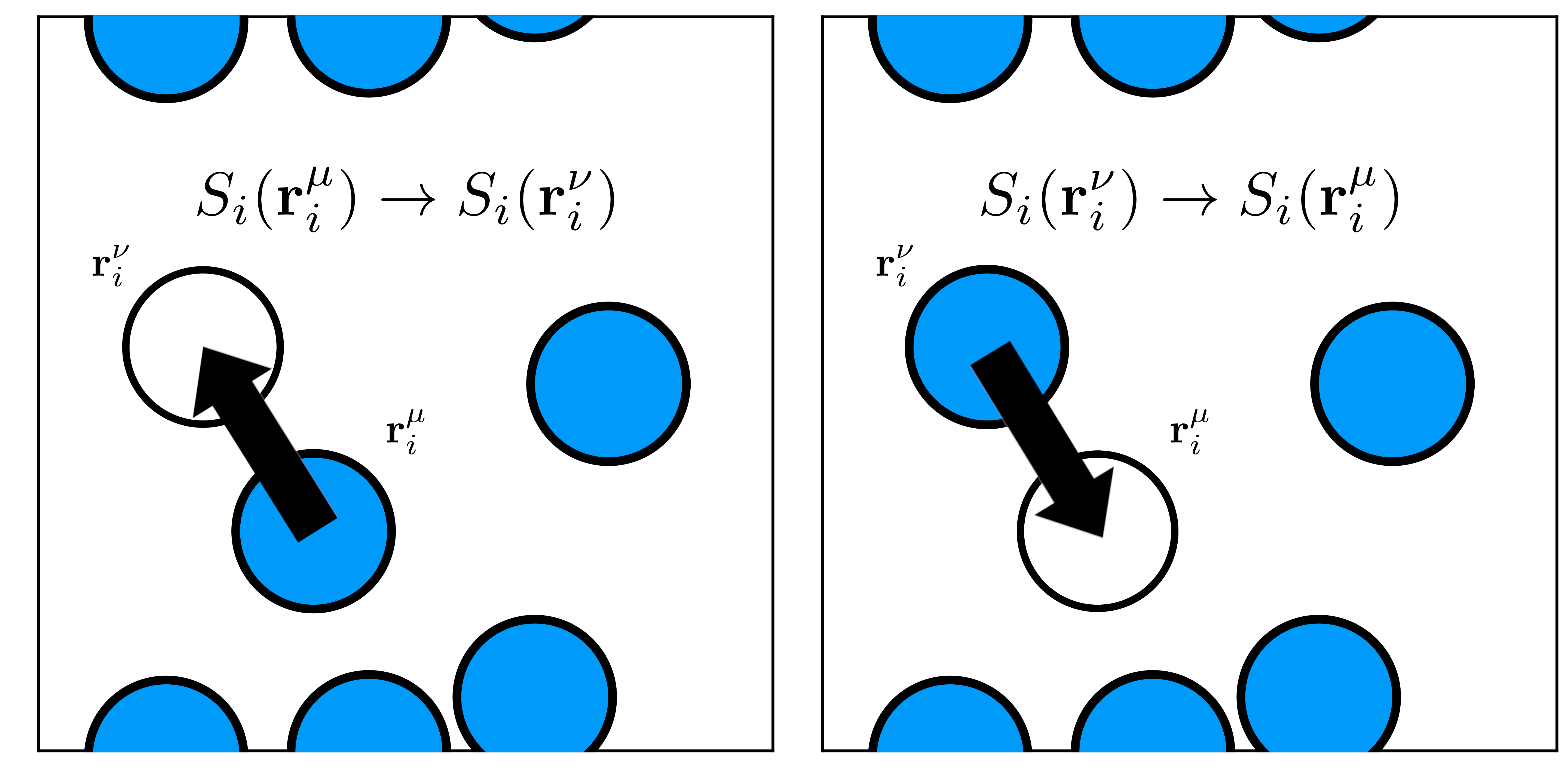
where the state $\nu$ is generated from state $\mu$ by displacing a molecule $i$ from $\vec{r}_i^\mu$ to $\vec{r}_i^\nu$. To ensure microscopic reversibility, the Metropolis method considers the probabilities of attempting the forward and reverse moves as equal.

Acceptance of this new state is subject to the probability:

$A(S_j \rightarrow S_i) = min(1, e^{-\beta(E_i - E_j)})$.

The algorithm is summarized in five simple steps:

1. Generation of an initial state. Particles should be uniformly distributed to avoid discontinuities in the potential energy.
2. Random selection of a particle $i$ with a random displacement given by $\vec{r}_i^{New} = \vec{r}_i^{Old} +\vec{\delta}_i(\vec{\eta - \frac{1}{2}})$.
3. Calcualte energy change $\Delta U = U(\vec{r}_N^{New}) - U(\vec{r}_N^{Old})$
   • If $\Delta U < 0$, the move is accepted.
   • If $\Delta U \geq 0$, a random number $\eta$ is chosen such that $0 \leq \eta \leq 1$.
     • If $\eta \leq e^{-\Delta U /k_BT}$ accept the move; else, reject it.
4. Sample therman and/or structural properties of interest.
5. Repeat fro step 2. until acceptable convergence criteria has been achieved.

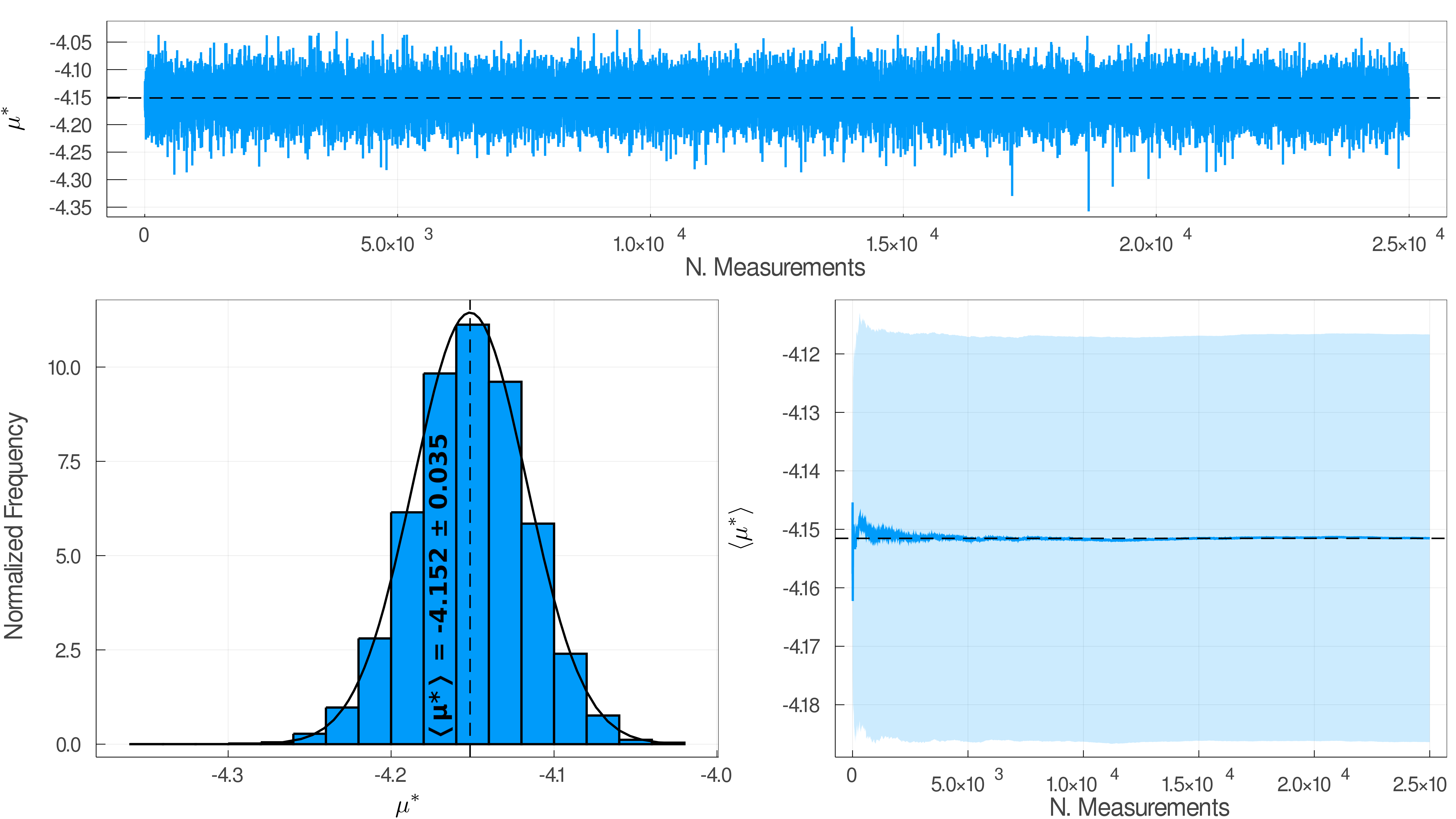
Code has been designed with succesful parameters as compared with official reported results. This includes a $20\sigma \times 20\sigma \times 20 \sigma$ simulation box with $2 \times N \times 10^4$ relaxation steps and $2.5 \times N \times 10^5$ equilibrium steps, for a total of 25,000 samples.

A simple and semi-interactive execution has been designed for those not familiar with the Julia language, where the density and temperature are taken as parameters, i. e., a system with $\rho^* = 0.1$ and $T^* = 1.5$:

1
    julia Canonical.jl 0.1 1.5

This generates output files with the energy, chemical potential and radial distribution function evolution of the system along the simulation, as well as their corresponding plots.

Code found at my personal github repository.